How Does Dengo Generate Solvers?
Contents
How Does Dengo Generate Solvers?
This tutorial tells you how the solver are generated with the help of dengo.ChemicalNetwork, and Jinja2. In short, dengo.ChemicalNetwork carries the full information of the chemical reactions and cooling actions of interest. It internally generates the symbolic representation of the dynamics of each chemical species. This can be exported as C++ or python code with a pre-written templates which can be found under dengo/templates. In this example we will be demonstrating how to generate rhs and solve the initial value problem withscipy.odeint
Import Libraries and Create the Network
Primordial rates and cooling for the 9-species network are included in the default dengo library in dengo.primordial_rates and dengo.primordial_cooling. The reactions and cooling are added automatically to the reaction_registry, cooling_registry and species_registry with the call to dengo.primordial_rates.setup_primordial.
Here we setup the same sample network we demonstrated in the last chapter with k01, k02 and reHII.
import dengo
from dengo.chemical_network import \
 ChemicalNetwork, \
 reaction_registry, \
 cooling_registry, species_registry
import dengo.primordial_rates
import dengo.primordial_cooling

dengo.primordial_rates.setup_primordial()

simpleNetwork = ChemicalNetwork()
simpleNetwork.add_reaction("k01")
simpleNetwork.add_reaction("k02")
simpleNetwork.add_cooling("reHII")
simpleNetwork.init_temperature((1e0, 1e8))
Adding reaction: k01 : 1*H_1 + 1*de => 1*H_2 + 2*de
Adding reaction: k02 : 1*H_2 + 1*de => 1*H_1
Building the solver
In this example, we will walk you through how to write a template from scratch that can be fed into a scipy solver. This can be done with ChemicalNetwork.write_solver and the combination of templates available under dengo/templates.
Evaluate the reaction rates
Reaction rates usually have a temperature dependence. For example, for reactions following the Arrhenius equation usually have the forms of \(k(T) = A e^{-\frac{E_a}{RT}}\), where \(k\) is the reaction rate, \(E_a\) is the activation energy of the reaction, \(T\) is the temperature, \(A\), \(R\) are the pre-exponential factor, and the universal gas constant respectively. \(A\) is sometimes depends further on temperature in Modified Arrhenius equation.
Evaluating these rates on the fly would be computationally expensive. One possible way of reducing the computational time is to interpolate from a pre-calculated reaction rates table. The rates are specified when the reactions rxn are first created with the @reaction decorator. They can be evaluated handily with rxn.coeff_fn(chemicalnetwork). The range of temperature of interest for example \(T = \rm (1, 10^8) K\) can be first specified with ChemicalNetwork.init_temperature(T_bounds=(1e0, 1e8), n_bins=1024). The added reaction objects can be accessed with ChemicalNetwork.reactions. For example, the reaction rates of k01 can the accessed with the snippet below
rxn_rate = cn.reactions['k01'].coeff_fn(ChemicalNetwork)
The output rxn_rate is an numpy array with a length of [n_bins].
A reaction rate table is generated and exported to a hdf5 file below.
with h5py.File(ofn, 'r') as f:
    print(f.keys())
>>> <KeysViewHDF5 ['T', 'k01', 'k02', 'reHII_reHII']>
import os
import h5py

solver_name = 'simple'
output_dir  = "."

ofn = os.path.join(output_dir, f"{solver_name}_tables.h5")

if os.path.exists(ofn):
    os.system(f"rm {ofn}")

with h5py.File(ofn, 'w') as f:
    for rxn in sorted(simpleNetwork.reactions.values()):
        f.create_dataset(
            f"/{rxn.name}", data=rxn.coeff_fn(simpleNetwork).astype("float64")
        )

    for rxn in sorted(simpleNetwork.cooling_actions.values()):
        if hasattr(rxn, "tables"):
            for tab in rxn.tables:
                f.create_dataset(
                    f"/{rxn.name}_{tab}",
                    data=rxn.tables[tab](simpleNetwork).astype("float64"),
                )
    f.create_dataset(f"/T", data=simpleNetwork.T.astype("float64"))
Using Jinja2
Jinja2 fills out variables dynamically with the user-given inputs. It is however not limited to variables subsitution. You can also use conditions (if/else), for loops (for), filter, and tests in Jinja2 template. To construct our solver template for scipy, we will be using for-loop, if-else, and variable substitution. And we will go through these usages briefly below their respective syntax. We refer our readers for more details in Jinja2 Documentation.
For example if the template is Dengo {{token}}, Jinja2 would look for the user-fed input for the variable token, and output the file with the word in curly bracket replaced with the token = "works".
from jinja2 import Template
t = Template("Dengo {{ token }}!")
print(t.render(token="works"))
Dengo works!
Jinja2 also provided an straightforward way to iterate over iterables like lists, with the syntax {% for item in list %} {% endfor %}. In the example below, we iterate over the required species in our chemical network, and had Jinja2 print out their name.
t = Template("""
{% for s in network.required_species | sort %}
{{s.name}},
{% endfor %}
""")
print(t.render(network = simpleNetwork))
H_1,

H_2,

de,

ge,
Preparing the rates interpolation template
In the template below, we demonstrate a simple implementation for interpolating reaction and cooling rates with Jinja2 and our ChemicalNetwork object. In brief, the template below first reads in the rates from the hdf5 we created above, and two functions interpolate_rates and interpolate_cooling_rates are created dynamically based on the reactions avaiable in our ChemicalNetwork.
reaction_rates_template = Template("""
import numpy as np
import h5py

# read rates in as global variables
rates_table = "{{solver_name}}_tables.h5"
ratef = h5py.File(rates_table, 'r')

# Reaction Rates
{% for k in network.reactions.keys()%}
out{{k}}dev = ratef['{{k}}'][:]
{%- endfor %}

# Cooling Rates
{%- for name, rate in network.cooling_actions | dictsort %}
{%- for name2 in rate.tables | sort %}
out_{{name}}_{{name2}} = ratef["{{name}}_{{name2}}"][:]
{%- endfor %}
{%- endfor %}
tdev = ratef['T'][:]
ratef.close()

def interpolate_rates(T):
    {% for k in network.reactions.keys()%}
    {{k}} = np.interp(T, tdev, out{{k}}dev)
    {%- endfor %}
    return (
    {%- for k in network.reactions.keys() -%}
    {{k}},
    {%- endfor -%}
    )
def interpolate_cooling_rates(T):
    {%- for name, rate in network.cooling_actions | dictsort %}
    {%- for name2 in rate.tables | sort %}
    {{name}}_{{name2}} = np.interp(T, tdev, out_{{name}}_{{name2}})
    {%- endfor %}
    {%- endfor %}
    return (
    {%- for name, rate in network.cooling_actions | dictsort -%}
    {%- for name2 in rate.tables | sort -%}
    {{name}}_{{name2}},
    {%- endfor -%}
    {%- endfor -%}
    )
    """)

template_vars = dict(
    network=simpleNetwork,
    solver_name=solver_name
)
output_file = f'{solver_name}_reaction_rate.py'
with open(output_file, 'w') as f:
    f.write(reaction_rates_template.render(template_vars))
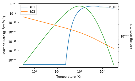
Import the Rendered simple_reaction_rate.py and Check if it works!
from simple_reaction_rate import interpolate_rates, interpolate_cooling_rates
import matplotlib.pyplot as plt

temperature = simpleNetwork.T
rxnk01_rate, rxnk02_rate = interpolate_rates(temperature)
coolreHII_rate,          = interpolate_cooling_rates(temperature)

plt.loglog(temperature, rxnk01_rate, label='k01')
plt.loglog(temperature, rxnk02_rate, label='k02')
plt.xlabel(r'Temperature $(\rm K)$')
plt.ylabel(r'Reaction Rate $(\rm g^{-1} cm^{3} s^{-1} )$')
plt.legend()
ax2 = plt.twinx()
ax2.loglog(temperature, coolreHII_rate,color='C2', label='reHII')
plt.ylabel(r'Cooling Rate reHII')
plt.legend()
<matplotlib.legend.Legend at 0x7efd3c629550>
Implement the temperature function
gamma = 5./3.
kb    = 1.38e-16
mh    = 1.67e-24

def calculate_temperature(state: npt.ArrayLike):
    # extract the abundance from the state vector
    {% for s in network.required_species | sort -%}
    {{s.name}},
    {%- endfor -%}
    = state
    density = {{network.print_mass_density()}}
    T = {{network.temperature_calculation()}}
    return T
temperature_template = Template("""
import numpy as np
gamma = 5./3.
kb    = 1.38e-16
mh    = 1.67e-24

def calculate_temperature(state):
    # extract the abundance from the state vector
    {% for s in network.required_species | sort -%}
    {{s.name}},
    {%- endfor -%}
    = state
    density = {{network.print_mass_density()}}
    T = {{network.temperature_calculation()}}
    return T


""")
output_file = f'{solver_name}_temperature.py'
with open(output_file, 'w') as f:
    f.write(temperature_template.render(network =simpleNetwork))
# %load simple_temperature.py

gamma = 5./3.
kb    = 1.38e-16
mh    = 1.67e-24

def calculate_temperature(state):
    # extract the abundance from the state vector
    H_1,H_2,de,ge,= state
    density = 1.0079400000000001*H_1 + 1.0079400000000001*H_2
    T = density*ge*mh/(kb*(H_1/(gamma - 1.0) + H_2/(gamma - 1.0) + de/(gamma - 1.0)))
    return T
# from simple_temperature import calculate_temperature
import numpy  as np
# Prepare the initial state vector
ge = 1e13  #erg/g
H_1 = 1e-2# 1/cm^3
H_2 = 1e-2# 1/cm^3
de  = 1e-2# 1/cm^3
state = np.array([H_1, H_2, de, ge])
simple_temperature.calculate_temperature(state)
---------------------------------------------------------------------------
NameError                                 Traceback (most recent call last)
Input In [9], in <cell line: 9>()
      7 de  = 1e-2# 1/cm^3
      8 state = np.array([H_1, H_2, de, ge])
----> 9 simple_temperature.calculate_temperature(state)

NameError: name 'simple_temperature' is not defined
Implement the RHS function
rhs_template = Template("""
import numpy as np
from {{solver_name}}_temperature import calculate_temperature
from {{solver_name}}_reaction_rate import interpolate_rates, interpolate_cooling_rates
mh    = 1.67e-24

def rhs_func(state, t):

    # extract the abundance from the state vector
    {% for s in network.required_species | sort -%}
    {{s.name}},
    {%- endfor -%}
    = state

    T   = calculate_temperature(state)[np.newaxis]

    {% for k in network.reactions.keys() -%}
    {{k}},
    {%- endfor -%}
    = interpolate_rates    (T)

    i = 0

    {% for name, rate in network.cooling_actions | dictsort -%}
    {%- for name2 in rate.tables | sort -%}
    {{name}}_{{name2}},
    {%- endfor -%}
    {%- endfor -%}
    = interpolate_cooling_rates(T)

    rho = {{network.print_mass_density()}}

    {% for s in network.required_species | sort %}
    {% if s.name != "ge" %}
    d{{s.name}}dt = {{network.species_total(s)}}
    {% else %}
    d{{s.name}}dt = {{network.print_cooling(assign_to=None)}} / mh/ rho
    {%- endif -%}
    {%- endfor %}

    return {% for s in network.required_species | sort -%}
    d{{s.name}}dt,
    {%- endfor -%}

""")

output_file = f'{solver_name}_rhs.py'
with open(output_file, 'w') as f:
    f.write(rhs_template.render(template_vars))
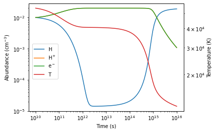
from simple_rhs import rhs_func
from scipy.integrate import odeint

timesteps = np.logspace(10, 16,101)
output     = odeint(rhs_func, state, t=timesteps)

H_1_traj, H_2_traj, de_traj, ge_traj = output.T

f, ax = plt.subplots()
l1= ax.loglog(timesteps, H_1_traj)
l2= ax.loglog(timesteps, H_2_traj)
l3= ax.loglog(timesteps, de_traj)
ax2 = ax.twinx()
T_traj = calculate_temperature(output.T)
l4= ax2.loglog(timesteps, T_traj, color='C3')


ax.set_ylabel(r"Abundance ($\rm cm^{-3}$)")
ax2.set_ylabel("Temperature (K)")

ax.set_xlabel("Time (s)")

f.legend(
    [l1,l2,l3,l4],
    labels=[r'$\rm H$',r'$\rm H^+$',r'$\rm e^-$',r'$\rm T$'],
    loc=[0.15,0.4]
)
plt.subplots_adjust(right=0.85)
/tmp/ipykernel_6081/297263008.py:23: UserWarning: You have mixed positional and keyword arguments, some input may be discarded.
  f.legend(

solver_rhs_template = Template("""
import h5py
import numpy as np
gamma = 5./3.
kb    = 1.38e-16
mh    = 1.67e-24


# read rates in as global variables
rates_table = "{{solver_name}}_tables.h5"
ratef = h5py.File(rates_table, 'r')

# Reaction Rates
{% for k in network.reactions.keys()%}
out{{k}}dev = ratef['{{k}}'][:]
{%- endfor %}

# Cooling Rates
{%- for name, rate in network.cooling_actions | dictsort %}
{%- for name2 in rate.tables | sort %}
out_{{name}}_{{name2}} = ratef["{{name}}_{{name2}}"][:]
{%- endfor %}
{%- endfor %}
tdev = ratef['T'][:]
ratef.close()

def interpolate_rates(T):
    {% for k in network.reactions.keys()%}
    {{k}} = np.interp(T, tdev, out{{k}}dev)
    {%- endfor %}
    return (
    {%- for k in network.reactions.keys() -%}
    {{k}},
    {%- endfor -%}
    )
def interpolate_cooling_rates(T):
    {%- for name, rate in network.cooling_actions | dictsort %}
    {%- for name2 in rate.tables | sort %}
    {{name}}_{{name2}} = np.interp(T, tdev, out_{{name}}_{{name2}})
    {%- endfor %}
    {%- endfor %}
    return (
    {%- for name, rate in network.cooling_actions | dictsort -%}
    {%- for name2 in rate.tables | sort -%}
    {{name}}_{{name2}},
    {%- endfor -%}
    {%- endfor -%}
    )


def calculate_temperature(state):
    # extract the abundance from the state vector
    {% for s in network.required_species | sort -%}
    {{s.name}},
    {%- endfor -%}
    = state
    density = {{network.print_mass_density()}}
    T = {{network.temperature_calculation()}}
    return T

def rhs_func(state, t):

    # extract the abundance from the state vector
    {% for s in network.required_species | sort -%}
    {{s.name}},
    {%- endfor -%}
    = state

    T   = calculate_temperature(state)[np.newaxis]

    {% for k in network.reactions.keys() -%}
    {{k}},
    {%- endfor -%}
    = interpolate_rates    (T)

    i = 0

    {% for name, rate in network.cooling_actions | dictsort -%}
    {%- for name2 in rate.tables | sort -%}
    {{name}}_{{name2}},
    {%- endfor -%}
    {%- endfor -%}
    = interpolate_cooling_rates(T)

    rho = {{network.print_mass_density()}}

    {% for s in network.required_species | sort %}
    {% if s.name != "ge" %}
    d{{s.name}}dt = {{network.species_total(s)}}
    {% else %}
    d{{s.name}}dt = {{network.print_cooling(assign_to=None)}} / mh/ rho
    {%- endif -%}
    {%- endfor %}

    return {% for s in network.required_species | sort -%}
    d{{s.name}}dt,
    {%- endfor -%}
""")

output_file = f'{solver_name}_solver.py'
with open(output_file, 'w') as f:
    f.write(solver_rhs_template.render(template_vars))
from simple_solver import rhs_func
timesteps = np.logspace(10, 16,101)
output     = odeint(rhs_func, state, t=timesteps)

H_1_traj, H_2_traj, de_traj, ge_traj = output.T

f, ax = plt.subplots()
l1= ax.loglog(timesteps, H_1_traj)
l2= ax.loglog(timesteps, H_2_traj)
l3= ax.loglog(timesteps, de_traj)
ax2 = ax.twinx()
T_traj = calculate_temperature(output.T)
l4= ax2.loglog(timesteps, T_traj, color='C3')


ax.set_ylabel(r"Abundance ($\rm cm^{-3}$)")
ax2.set_ylabel("Temperature (K)")

ax.set_xlabel("Time (s)")

f.legend(
    [l1,l2,l3,l4],
    labels=[r'$\rm H$',r'$\rm H^+$',r'$\rm e^-$',r'$\rm T$'],
    loc=[0.15,0.4]
)
plt.subplots_adjust(right=0.85)
/tmp/ipykernel_6081/2565928376.py:20: UserWarning: You have mixed positional and keyword arguments, some input may be discarded.
  f.legend(
Yay! you have learnt how to write a Jinja2 template from scratch
this template is also available under dengo/templates/scipy/dengo_rhs.py.template. While we only demonstrated it with a 2 species model with 2 reactions and 1 cooling action. This would still work for any user-specied network!
The workflow we outlined in this chapter works for a simple prototyping with scipy.integrate.odeint. To extend it to more efficient deployments with C libraries and the ODE solver SUNDIALS CVODE in massively parallel setting, we have also provide our template function for generating compilable C-libraries under dengo/templates/. This will be introduced in the next chapter.