Building A ODE solver
Contents
Building A ODE solver
We have created a ChemicalNetwork with 2 reactions and 1 cooling action. Now we are ready to put together an ODE solver to study the evolution of this chemical network with different initial conditions.
The dynamics of the system is specified by the set of ODE equations.
$\( \frac{d \bf y}{dt} = f(\bf y) \)\(
where \)\bf y\( corresponds to the abundance vector for the species of interest, and \)f(\bf y)\( describes the dynamics. \)\bf y$ in this case is [H_1, H_2, de, ge].
In the below, we will outline how can dengo help you with putting together the RHS function below and building a ODE solver.
$\(
\begin{align*}
\rm \frac{d H}{dt} &= \rm k_{02}(T) \, H^+ \, e^- - k_{01}(T) \, H \, e^- \\
\rm \frac{d H^+}{dt} &= \rm - k_{02}(T) \, H^+ \, e^- + k_{01}(T) \, H \, e^- \\
\rm \frac{d e^-}{dt} &= \rm - k_{02}(T) \, H^+ \, e^- + k_{01}(T) \, H \, e^- \\
\rm \frac{d ge}{dt} &= \rm - reHII(T) \, H^+ \, e^-
\end{align*}
\)$
This can be broken down into 3 different steps.
Evalulate temperature from the state vector
Evalulate/ Interpolate the reaction rates from the temperature
Evalulate the RHS function
Feed the RHS function into an ODE solver
Import Libraries and Create the Network
Primordial rates and cooling for the 9-species network are included in the default dengo library in dengo.primordial_rates and dengo.primordial_cooling. The reactions and cooling are added automatically to the reaction_registry, cooling_registry and species_registry with the call to dengo.primordial_rates.setup_primordial. Here we setup the same sample network we demonstrated in the last chapter with k01, k02 and reHII.
import dengo
from dengo.chemical_network import \
 ChemicalNetwork, \
 reaction_registry, \
 cooling_registry, species_registry
import dengo.primordial_rates
import dengo.primordial_cooling

dengo.primordial_rates.setup_primordial()

simpleNetwork = ChemicalNetwork()
simpleNetwork.add_reaction("k01")
simpleNetwork.add_reaction("k02")
simpleNetwork.add_cooling("reHII")
simpleNetwork.init_temperature((1e0, 1e8))
Adding reaction: k01 : 1*H_1 + 1*de => 1*H_2 + 2*de
Adding reaction: k02 : 1*H_2 + 1*de => 1*H_1
Evaluate the temperature
The temperature \(T\) as we have seen above is critical to the rate at which the reaction proceeds. The temperature can be evaluated from the internal energy term ge.
Internal energy of an ideal gas is:
$\( E = \rho \epsilon = c_V T = \frac{nkT}{\gamma -1}\)\(
For monoatomic gas \)\gamma\( is \)5/3\(, and diatomic gas \)\gamma\( is \)7/5\(. \)\gamma\( refers to the adiabatic constant, and it is directly related to the degree of freedom available to the species \)f = \frac{2}{\gamma -1}\(. When the temperature is higher, other degrees of freedom might get excited, and which leads toa temperature-dependent \)\gamma$.
The total internal energy in the mixture of ideal gas is: $\(\epsilon = \sum_s \frac{n_s kT}{\gamma_s -1}\)\(. \)T\( can be thus be calculated from \)E\( and the abundance of all the avaialble species \)n_s$.
In our simple example, the internal energy can be written out plainly as
Dengo can generate the sympy expression of \(\Gamma_{\rm eff}\) with the function ChemicalNetwork.gamma_factor(). We are at the position to define our our function to calculate the temperature, with the expression provided to us by Dengo. Notice that in Dengo, the internal energy term \(ge\) is treated as energy per unit mass density \(\epsilon = E/\rho\). You also ask Dengo to directly spit out the expression for temperature with simpleNetwork.temperature_calculation().
simpleNetwork.gamma_factor()
sorted(simpleNetwork.required_species)
[Species: H_1, Species: H_2, Species: de, Species: ge]
simpleNetwork.print_mass_density()
'1.0079400000000001*H_1 + 1.0079400000000001*H_2'
import numpy.typing as npt

gamma = 5./3.
kb    = 1.38e-16
mh    = 1.67e-24

def calculate_temperature(state: npt.ArrayLike):
    """calculate temperature in (K) based on the state space vector"""

    # extract the abundance from the state vector
    H_1, H_2, de, ge = state
    inv_gammam1 = 1 / (gamma - 1)
    gamma_factor = (H_1 + H_2 + de) * inv_gammam1
    rho = 1.00794*H_1 + 1.00794*H_2
    T = ge / gamma_factor / kb * mh * rho
    return T
Evaluate the reaction rates
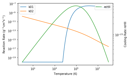
Evaluating these rates on the fly would be computationally expensive. One possible way of reducing the computational time is to interpolate from a pre-calculated reaction rates table. The rates are specified when the reactions rxn are first created with the @reaction decorator. They can be evaluated handily with rxn.coeff_fn(chemicalnetwork). The range of temperature of interest for example \(T = \rm (1, 10^8) K\) can be first specified with ChemicalNetwork.init_temperature(T_bounds=(1e0, 1e8), n_bins=1024).
# The reactions in the chemical network can be assessed
import numpy as np
import matplotlib.pyplot as plt
reactions = simpleNetwork.reactions
cooling   = simpleNetwork.cooling_actions

rxnk01 = reactions['k01']
rxnk02 = reactions['k02']
reHII  = cooling['reHII']
temperature = simpleNetwork.T
rxnk01_rate = rxnk01.coeff_fn(simpleNetwork)
rxnk02_rate = rxnk02.coeff_fn(simpleNetwork)

plt.loglog(temperature, rxnk01_rate, label='k01')
plt.loglog(temperature, rxnk02_rate, label='k02')
plt.xlabel(r'Temperature $(\rm K)$')
plt.ylabel(r'Reaction Rate $(\rm g^{-1} cm^{3} s^{-1} )$')
plt.legend()
ax2 = plt.twinx()
coolreHII_rate = reHII.tables['reHII'](simpleNetwork)
ax2.loglog(temperature, coolreHII_rate,color='C2', label='reHII')
plt.ylabel(r'Cooling Rate reHII')
plt.legend()
<matplotlib.legend.Legend at 0x7fe5133b6fd0>
logT       = np.log10(temperature)
k01lograte = np.log10(rxnk01_rate)
k02lograte = np.log10(rxnk02_rate)
coolreHII_lograte = np.log10(coolreHII_rate)

def interpolate_rates(T: npt.ArrayLike):
    """interpolate the reaction rate in log space

    Parameters
    ----------
        T: the temperate at which the rate is evaluated

    Return
    ------
        k02: interpolated reaction rate at temperature T
    """
    k01 = 10**np.interp(np.log10(T), logT, k01lograte)
    k02 = 10**np.interp(np.log10(T), logT, k02lograte)
    return k01, k02

def interpolate_cooling_rates(T: npt.ArrayLike):
    """interpolate the cooling rate in log space

    Parameters
    ----------
        T: the temperate at which the rate is evaluated

    Return
    ------
        coolreHII_rate: interpolated cooling rate at temperature T
    """
    coolreHII_rate = 10**np.interp(np.log10(T), logT, coolreHII_lograte)
    return coolreHII_rate
The RHS function
The dynamics is specified by the set of ODE equations. $\( \frac{d \bf y}{dt} = f(\bf y) \)\( where \)\bf y\( corresponds to the abundance vector for the species of interest, and \)f(\bf y)$ describes the dynamics.
Dengo aggreates the reactions specific to each species \(s\) with ChemicalNetwork.species_total(s) with sympy internally. These sympy expression can be exported to various different code style with sympy.printing to C, python for example.
for s in sorted(simpleNetwork.required_species):
    if s.name != 'ge':
        print(f"d{s.name:>3}dt = {simpleNetwork.species_total(s)}")
    else:
        print(f"d{s.name:>3}dt = {simpleNetwork.print_cooling(assign_to=None)}")
dH_1dt = -k01[i]*H_1*de + k02[i]*H_2*de
dH_2dt = k01[i]*H_1*de - k02[i]*H_2*de
d dedt = k01[i]*H_1*de - k02[i]*H_2*de
d gedt = -reHII_reHII[i]*H_2*de
def rhs_func(state, t):
    """evaluate the dydt given the state y at time t

    Parameters
    ----------
        state: np.ndarray
            the number density of different species
        t: float
            time
    Return
    ------
        coolreHII_rate: interpolated cooling rate at temperature T
    """
    H_1, H_2, de, ge = state

    T   = calculate_temperature(state)
    k01, k02 = interpolate_rates    (T)
    rho = 1.00794*H_1 + 1.00794*H_2

    reHII_reHII = interpolate_cooling_rates(T)

    dH_1dt = k02*H_2*de - k01*H_1*de
    dH_2dt = -k02*H_2*de + k01*H_1*de
    ddedt = -k02*H_2*de + k01*H_1*de
    dgedt = (-reHII_reHII*H_2*de)/ rho /mh

    dstatedt = np.array([dH_1dt,dH_2dt,ddedt,dgedt])
    return dstatedt
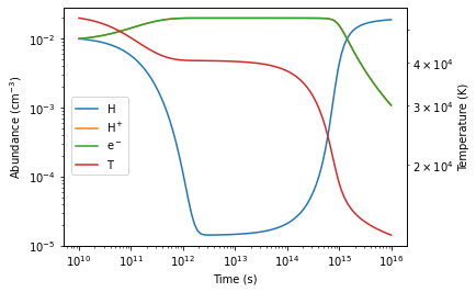
Integrate the System
Once the RHS function is specified, we are ready to evolve the system. Here we will use the scipy.integrate.odeint to integrate the ODE. The initial value are specified below as a 1D-vector. And the output logarithmically-spaced timesteps are also fed into the ODE solver.
# Prepare the initial state vector
ge = 1e13  #erg/g
H_1 = 1e-2# 1/cm^3
H_2 = 1e-2# 1/cm^3
de  = 1e-2# 1/cm^3
state = np.array([H_1, H_2, de, ge])
from scipy.integrate import odeint

timesteps = np.logspace(10, 16,101)
output     = odeint(rhs_func, state, t=timesteps)
H_1_traj, H_2_traj, de_traj, ge_traj = output.T

f, ax = plt.subplots()
l1= ax.loglog(timesteps, H_1_traj)
l2= ax.loglog(timesteps, H_2_traj)
l3= ax.loglog(timesteps, de_traj)
ax2 = ax.twinx()
T_traj = calculate_temperature(output.T)
l4= ax2.loglog(timesteps, T_traj, color='C3')


ax.set_ylabel(r"Abundance ($\rm cm^{-3}$)")
ax2.set_ylabel("Temperature (K)")

ax.set_xlabel("Time (s)")

f.legend(
    [l1,l2,l3,l4],
    labels=[r'$\rm H$',r'$\rm H^+$',r'$\rm e^-$',r'$\rm T$'],
    loc=[0.15,0.4]
)
plt.subplots_adjust(right=0.85)
/tmp/ipykernel_30087/3292852106.py:21: UserWarning: You have mixed positional and keyword arguments, some input may be discarded.
  f.legend(
Summary
We have built a reaction chemical network with 2 reactions and 1 cooling action from scratch with
Dengo!We demonstrated how can we build a simple ODE solver with the symbolic outputs from
Dengo!
In the next chapter, we demonstrate how Dengo can be used in conjunction with Jinja2 to write a solver for arbitary network in the next chapter.